Imagine you have data from two distinct clusters, each with 200
features and 50 observations. The interesting part: only 10% of these
features (20 features) actually differ between the groups. The remaining
features are identically distributed. The magnitude of these differences
is controlled by a parameter called delta.
Generating Example Data
Let’s create such a dataset using the gen_data_normal
function:
data = gen_data_normal(n = 100, p = 200, prop = 0.1, delta = 3)
X = data$X
L = data$L
In this example:
- Features 1 through 20 are truly different between clusters
(
delta = 3) - Features 21 through 200 are identically distributed (no difference)
Identifying Non-null Features by DS
Now, let’s use our DS procedure to automatically identify which
features distinguish the two clusters while controlling the false
discovery rate (FDR) at a nominal level of q = 0.2:
Evaluating Performance
We know the ground truth: features 1–20 are truly different. Let’s measure how accurately DS identified them:
calc_acc(res$sel_set, 1:20)
#>        fdr      power         f1
#> 0.04761905 1.00000000 0.97560976
This gives us:
- Precision (1 - FDR): Proportion of selected features that are truly different
- Recall (Power): Proportion of true features that were correctly identified
- F1 score: Harmonic mean of precision and recall
Visualizing Mirror Statistics
DS uses mirror statistics to distinguish signal from noise. Let’s visualize their distribution:
hist(res$ms)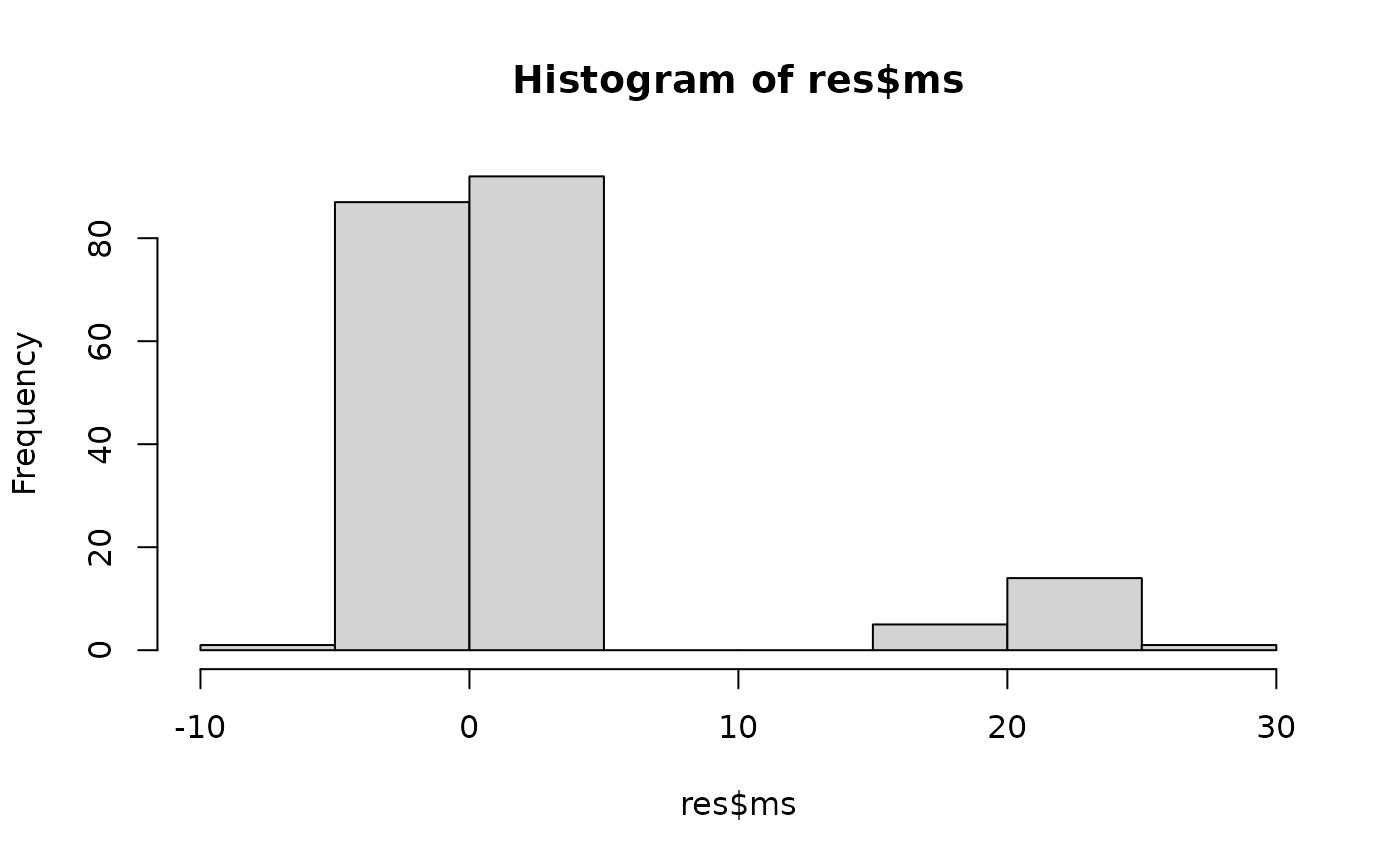
Interpretation: Mirror statistics with large positive values suggest strong evidence of differences between clusters.
A More Robust Approach: MDS
For increased robustness against variability, you can use the MDS (Multiple DS) procedure, which aggregates results across multiple random splits:
Check the accuracy of the selected set
calc_acc(res, 1:20)
#>   fdr power    f1
#>     0     1     1
💡 Key Takeaways
- DS provides a straightforward approach to feature selection with FDR control
- MDS offers enhanced robustness through aggregation across multiple random splits
- Both methods aim to identify the 20 truly different features while controlling false discoveries
- The histogram of mirror statistics helps visualize the separation between signal and noise